Mouse embryo scNMT-seq data

Here we use a multi-omics scNMT-seq dataset to demonstrate the simple usage of MultiSpace. The scNMT-seq data was derived from the study of early mouse embryo (Argelaguet et al., Nature, 2019). From E4.5 to E7.5 are used in this example. The spatial data was collected from E8.5 mouse embryo (Lohoff et al., Nature, 2022).

Using MultiSpace to analysis

Take E8.5 scNMT-seq data for example. Users should better separate data in absolute folder if they have more than one stage.

Step 1 Run MultiSpace Pipelineinit to initialize snakemake

The first step of running MultiSpace pipeline is to initialize pipeline config file (also initiation sample in same file)and a working directory. All these steps are implemented by :bash:`MultiSpace Pipelineinit` function.

MultiSpace Pipelineinit --species mm10 \
--samplesheet metasheet.csv \
--directory ~/Project/scNMT_WolfReik/ \
--fasta ~/Reference/mm10.fa \
--fasta_fai ~/Reference/mm10.fa.fai \
--lambda_fasta ~/Reference/mm10_lambda.fa \
--star_annotation ~/Reference/UCSC_mm10/mm10.refGene.gtf \
--star_index ~/Reference/UCSC_mm10/

The results of :bash:`MultiSpace Pipelineinit` are shown as below.

File	Description
config.yaml	Initialized config.yaml generated in user input directory.
Snakefile	Snakefile in directory used for running snakemake.
modules/	Snakemake rules stored in subdir modules of directory.

Step 2 Run snakemake to preprocess raw data

After initialize config file and working directory, :bash:`snakemake -j 5` could be used to run snakemake in working directory. Users can customize cores number ,but be careful not to make the number too large in case limited memory.

cd ~/Project/scNMT_WolfReik/
snakemake -j 5

The results of :bash:`snakemake -j 5` are shown as below. DNA methylation(WCG, W=A or T). Chromatin accessibility(GCH, H=A, C or T)

File	Description
GCH.bin_peak.h5	GCH bin by cell marix stored in H5 format.
WCG.bin_peak.h5	WCG bin by cell marix stored in H5 format.
GCH.bin.merge.peak	GCH bin features. Rowname of GCH.bin_peak.h5
WCG.bin.merge.peak	WCG bin features. Rowname of WCG.bin_peak.h5
GCH.chr1_chr6.site_peak.h5 GCH.chr7_chr12.site_peak.h5 GCH.chr13_chrY.site_peak.h5	GCH site by cell matrix separated by chromatin stored in H5 format.
WCG.site_peak.h5	WCG site by cell matrix stored in H5 format.
WCG.uniq.peak	WCG site features. Rowname of WCG.site_peak.h5
GCH.uniq.peak	GCH site features. Rowname of GCH.site_peak.h5(merge chromtain together)
QCtable.txt	Snakemake rules stored in subdir modules of directory.
usecell.txt	Snakemake rules stored in subdir modules of directory.
QCtable.txt	Snakemake rules stored in subdir modules of directory.

Step 3 Run MultiSpace Scorematrix to calculate WCG/GCH score matrix

MultiSpace Scorematrix can calculate genebody or gene promoter methylation ratio using snakemake output file.

MultiSpace Scorematrix --species mm10 --cell_barcode 04.WCG.GCH/usecell.txt \
--file_path 04.WCG.GCH/ --outdir . --matrixtype WCG --region promoter --distance 2000

The results of :bash:`MultiSpace Scorematrix` are gene by cell matrix stored in TXT format.

MultiSpace Scorematrix can calculate gene activity score using RP(regulatory potential) model.

MultiSpace Scorematrix --species mm10 --cell_barcode 04.WCG.GCH/usecell.txt \
--file_path 04.WCG.GCH/ --outdir . --matrixtype GCH --distance 10000

The results of :bash:`MultiSpace Scorematrix` are gene by cell matrix stored in TXT format.

Step 4 Run MultiSpace Mappingcell to map single cell to spatial

MultiSpace Mappingcell can map single cell to spatial location, and get spatially epigenetic signal. Users can take :bash:`snakemake` output single cell gene expression matrix, bin by cell matrix and bin features as input. Additionally, users should offer a spatial gene count matrix and cell type file. The count matrix could be tab-separated plain-text file with genes as rows and spots as columns. The celltype file should be a tab-separated plain-text file without header. The first column should be the cell name, and the second column should be the corresponding celltype labels.

MultiSpace Mappingcell --sc_count_file 05.Spatial/RNA_normalized.txt --sc_celltype_file celltype.txt \
--st_count_file Spatial/seqFISH_scRNA/RNA_st_normalized.txt --spatial_location Spatial/seFISH_scRNA/loc_EM1.txt \
--epi_binfile WCG.bin_peak.h5 --epi_feature WCG.bin.merge.peak --out_dir . --out_prefix WCG

Users can use :bash:`MultiSpace Mappingcell --help` to see help message. The results are showed below.

File	Description
WCG.signal_mat.npz	DNA methylation signal in spatila location. Bin feature by spot matrix stored in .npz format.
WCG.signal_mat_rowname.txt	Rownames of bin feature by spot matrix after filtering. Colnames of bin feature by spot matrix is colnames of st_count_file.

Validate mapping accuracy:

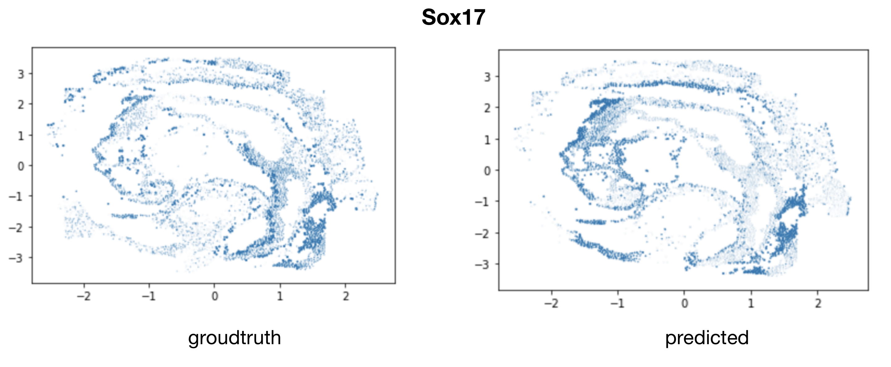
Mapping E7.5 scNMT-seq data to E8.5 spatial location:

MultiSpace output file downstream analysis

Users can use :bash:`snakemake` output file to do downstream analysis.

Single omic clustering

Using Seurat to cluster RNA gene count matrix by stage and celltype.

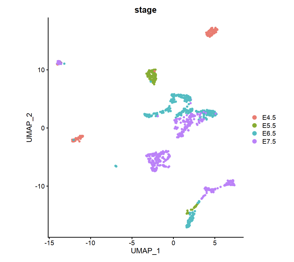
Mouse embryo gene count matrix cluster by stage(from E4.5 to E7.5)

library(Seurat)
library(ggplot2)
library(patchwork)
library(dplyr)
library(data.table)
library(stringr)
samplemeta = read.table("allsamplemeta.txt",sep = " ", header = T)
RNA_mat <- as.data.frame(read.table("RNA_normalized.txt",header = T,row.names = 1, check.names=FALSE))

scseurat <- CreateSeuratObject(
 counts = RNA_mat,
 project = "RNA",
 assay = "RNA",
 min.cells = 5
)
scseurat@meta.data$type <- "rna"
scseurat@meta.data$sample <- rownames(scseurat@meta.data)
scseurat@meta.data = merge(samplemeta,scseurat@meta.data,on = "sample")
rownames(scseurat@meta.data) = scseurat@meta.data$sample

scseurat <- NormalizeData(scseurat) %>% ScaleData()
scseurat <- SCTransform(scseurat, assay = "RNA",  verbose = FALSE)
scseurat <- RunPCA(scseurat, dims = 1:30)
scseurat <- RunUMAP(scseurat, dims = 1:30)
scseurat <- FindNeighbors(scseurat, dims = 1:30)
scseurat <- FindClusters(scseurat, resolution = 0.5, verbose = FALSE)

DimPlot(scseurat,reduction = "umap",group.by = "stage")

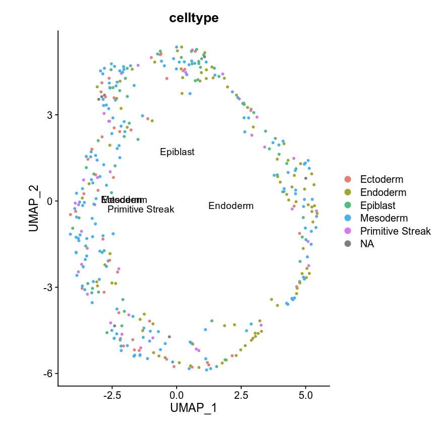
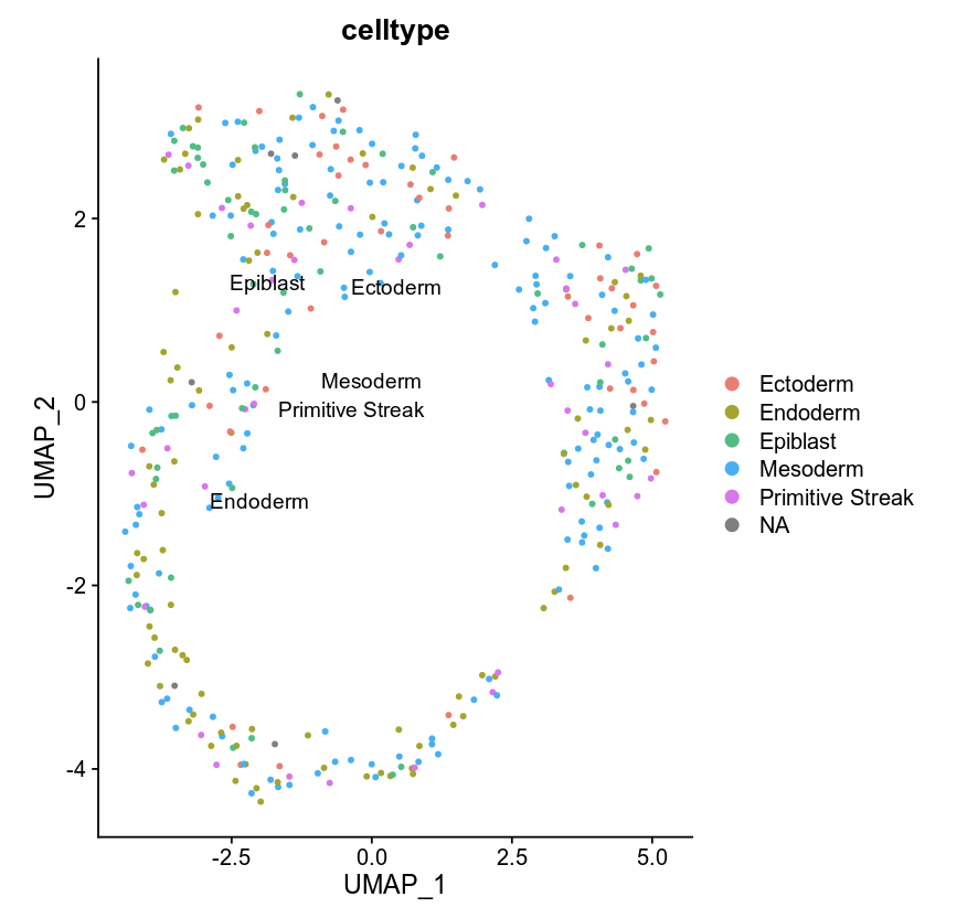
Mouse embryo gene count matrix cluster by celltype in E7.5.

e75samplemeta = samplemeta[which(samplemeta$stage == "E7.5"),]
e75RNA_mat = RNA_mat[,which(colnames(RNA_mat) %in% e75samplemeta$sample)]

e75scseurat <- CreateSeuratObject(
 counts = e75RNA_mat,
 project = "RNA",
 assay = "RNA",
 min.cells = 3
)
e75scseurat@meta.data$type <- "rna"
e75scseurat@meta.data$orig.ident <- "E7.5"
e75scseurat@meta.data$sample <- rownames(e75scseurat@meta.data)
e75scseurat@meta.data = merge(samplemeta,e75scseurat@meta.data,on = "sample")
rownames(e75scseurat@meta.data) = e75scseurat@meta.data$sample

e75scseurat <- SCTransform(e75scseurat, assay = "RNA",  verbose = FALSE)
e75scseurat <- RunPCA(e75scseurat, dims = 1:30)
e75scseurat <- RunUMAP(e75scseurat, dims = 1:30)
e75scseurat <- FindNeighbors(e75scseurat, dims = 1:30)
e75scseurat <- FindClusters(e75scseurat, resolution = 0.5, verbose = FALSE)

DimPlot(e75scseurat,reduction = "umap",group.by = "celltype")

Using Signac to cluster WCG/GCH bin count matrix by stage(from E4.5 to E7.5). Take WCG bin matrix for example.

library(Signac)
library(Seurat)
library(ggplot2)
library(stringr)
library(reticulate)
library(Matrix)
np <- import("numpy")
scipy <-import("scipy")

feature = read.csv("WCG.bin.merge.peak",header = F)
usecell <- read.table("usecells.txt")
mydata <- h5read("WCG.bin_peak.h5", "Mcsc")
WCG_mat = sparseMatrix(x = as.numeric(mydata$data),j = as.numeric(mydata$indices),p = as.numeric(mydata$indptr),dims = c(4114260,985),index1 = FALSE)
colnames(WCG_mat) = usecell$V1
rownames(WCG_mat) = feature$V1
meta <- read.table("sample_metadata.txt",sep = "\t", header = T)
samplemeta = merge(meta,usecell, by.x = "sample",by.y = "V1")[,c('sample','stage','lineage10x')]
rownames(samplemeta) = samplemeta$sample
samplemeta$celltype = samplemeta$lineage10x

WCG <- CreateSeuratObject(
 counts = WCG_mat,
 assay = "peaks",
 min.cells = 5,
 meta = samplemeta
)
WCG@meta.data$celltype = samplemeta$celltype

WCG <- RunTFIDF(WCG)
WCG <- FindTopFeatures(WCG, min.cutoff = "q90")
WCG <- RunSVD(WCG)
WCG <- RunUMAP(
  object = WCG,
  reduction = 'lsi',
  dims = 2:20
)

DimPlot(object = WCG, label = TRUE, reduction = "umap", group.by = "stage")

Using Signac to cluster WCG/GCH bin count matrix by celltype in E7.5.

e75samplemeta = samplemeta[which(samplemeta$stage == "E7.5"),]
WCG_mat = WCG_mat[,e75samplemeta$sample]
e75WCG <- CreateSeuratObject(
 counts = WCG_mat,
 assay = "peaks",
 min.cells = 3,
 meta = e75samplemeta
)
e75WCG@meta.data$celltype = e75samplemeta$celltype

e75WCG <- RunTFIDF(e75WCG)
e75WCG <- FindTopFeatures(e75WCG, min.cutoff = "q90")
e75WCG <- RunSVD(e75WCG)
e75WCG <- RunUMAP(
  object = e75WCG,
  reduction = 'lsi',
  dims = 2:20
)

DimPlot(object = e75WCG, label = TRUE, reduction = "umap", group.by = "celltype")

Multi omics clustering

library(reticulate)
library(Seurat)
library(Signac)
library(dplyr)
library(ggplot2)
library(rhdf5)
library(Matrix)
np <- import("numpy")
scipy <-import("scipy")
h5py <- import("h5py")

meta <- read.table("sample_metadata.txt",sep = "\t", header = T)
usecell <- read.table("usecells.txt")
samplemeta = merge(meta,usecell, by.x = "sample",by.y = "V1")[,c('sample','stage','lineage10x')]
rownames(samplemeta) = samplemeta$sample
samplemeta$celltype = samplemeta$lineage10x

RNA_mat <- as.data.frame(read.table("RNA_normalized.txt",header = T,row.names = 1, check.names=FALSE))

wcgfeature = read.csv("WCG.bin.merge.peak",header = F)
mydata <- h5read("WCG.bin_peak.h5", "Mcsc")
WCG_mat = sparseMatrix(x = as.numeric(mydata$data),j = as.numeric(mydata$indices),p = as.numeric(mydata$indptr),dims = c(4114260,985),index1 = FALSE)
colnames(WCG_mat) = usecell$V1
rownames(WCG_mat) = wcgfeature$V1

gchfeature = read.csv("GCH.bin.merge.peak",header = F)
mydata <- h5read("GCH.bin_peak.h5", "Mcsc")
GCH_mat = sparseMatrix(x = as.numeric(mydata$data),j = as.numeric(mydata$indices),p = as.numeric(mydata$indptr),dims = c(2645763,985),index1 = FALSE)
colnames(GCH_mat) = usecell$V1
rownames(GCH_mat) = gchfeature$V1

seurat <- CreateSeuratObject(
 counts = RNA_mat,
 project = "RNA",
 assay = "RNA",
 metadata = samplemeta,
 min.cells = 5
)
seurat[['WCG']] <- CreateAssayObject(counts = WCG_mat,min.cells = 10)
seurat[['GCH']] <- CreateAssayObject(counts = GCH_mat,min.cells = 10)
seurat@meta.data <- cbind(seurat@meta.data,samplemeta)

# RNA analysis
DefaultAssay(seurat) <- "RNA"
seurat <- SCTransform(seurat, verbose = FALSE) %>% RunPCA() %>% RunUMAP(dims = 1:50, reduction.name = 'umap.rna', reduction.key = 'rnaUMAP_')

# WCG analysis
# We exclude the first dimension as this is typically correlated with sequencing depth
DefaultAssay(seurat) <- "WCG"
seurat <- RunTFIDF(seurat)
seurat <- FindTopFeatures(seurat, min.cutoff = 'q90')
seurat <- RunSVD(seurat)
seurat <- RunUMAP(seurat, reduction = 'lsi', dims = 2:50, reduction.name = "umap.wcg", reduction.key = "wcgUMAP_")

# GCH analysis
# We exclude the first dimension as this is typically correlated with sequencing depth
DefaultAssay(seurat) <- "GCH"
seurat <- RunTFIDF(seurat)
seurat <- FindTopFeatures(seurat, min.cutoff = 'q90')
seurat <- RunSVD(seurat)
seurat <- RunUMAP(seurat, reduction = 'lsi', dims = 2:50, reduction.name = "umap.gch", reduction.key = "gchUMAP_")


DefaultAssay(seurat) <- "RNA"
seurat <- FindMultiModalNeighbors(seurat, reduction.list = list("pca", "lsi","lsi"), dims.list = list(1:50, 2:50, 2:50))
seurat <- RunUMAP(seurat, nn.name = "weighted.nn", reduction.name = "wnn.umap", reduction.key = "wnnUMAP_")
seurat <- FindClusters(seurat, graph.name = "wsnn", algorithm = 3, verbose = FALSE)

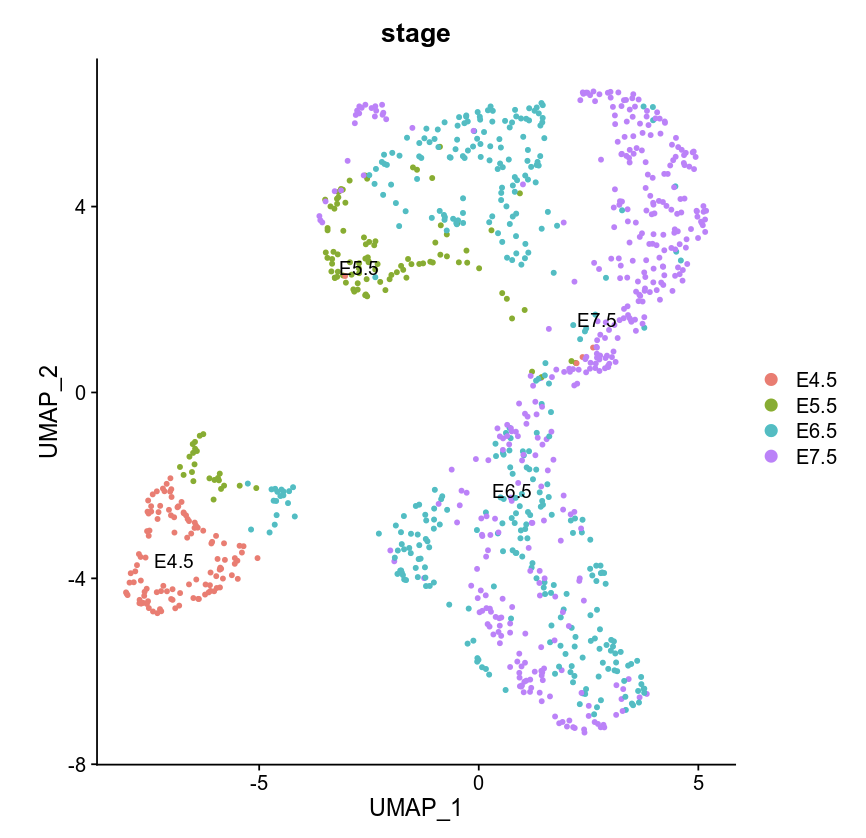
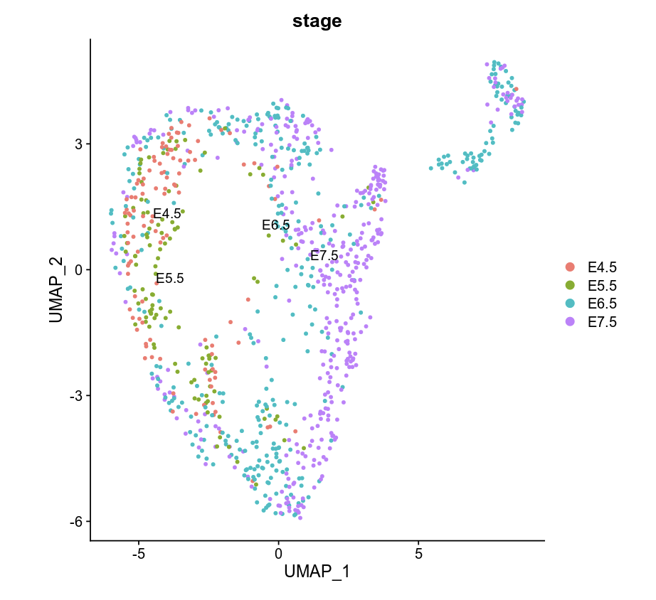
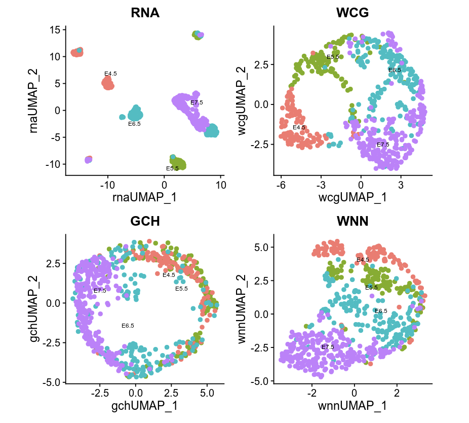
p1 <- DimPlot(seurat, reduction = "umap.rna", group.by = "stage", label = TRUE, label.size = 2.5, pt.size = 2, repel = TRUE) + ggtitle("RNA")
p2 <- DimPlot(seurat, reduction = "umap.wcg", group.by = "stage", label = TRUE, label.size = 2.5, pt.size = 2, repel = TRUE) + ggtitle("WCG")
p3 <- DimPlot(seurat, reduction = "umap.gch", group.by = "stage", label = TRUE, label.size = 2.5, pt.size = 2, repel = TRUE) + ggtitle("GCH")
p4 <- DimPlot(seurat, reduction = "wnn.umap", group.by = "stage", label = TRUE, label.size = 2.5, pt.size = 2, repel = TRUE) + ggtitle("WNN")
p1 + p2 + p3 +p4 & NoLegend() & theme(plot.title = element_text(hjust = 0.5))

E75meta <- samplemeta[samplemeta$stage == "E7.5" & samplemeta$celltype %in% c("Endoderm","Ectoderm","Mesoderm"),]
RNA_mat <- RNA_mat[,E75meta$sample]
seurat <- CreateSeuratObject(
 counts = RNA_mat,
 project = "RNA",
 assay = "RNA",
 metadata = E75meta,
 min.cells = 3
)
seurat@meta.data <- cbind(seurat@meta.data,E75meta)
GCH_mat <- GCH_mat[,E75meta$sample]
seurat[['GCH']] <- CreateAssayObject(counts = GCH_mat,min.cells = 5)
WCG_mat <- WCG_mat[,E75meta$sample]
seurat[['WCG']] <- CreateAssayObject(counts = WCG_mat,min.cells = 5)

# RNA analysis
DefaultAssay(seurat) <- "RNA"
seurat <- SCTransform(seurat, verbose = FALSE) %>% RunPCA() %>% RunUMAP(dims = 1:50, reduction.name = 'umap.rna', reduction.key = 'rnaUMAP_')
#Note that this single command replaces NormalizeData(), ScaleData(), and FindVariableFeatures()
# GCH analysis
# We exclude the first dimension as this is typically correlated with sequencing depth
DefaultAssay(seurat) <- "GCH"
seurat <- RunTFIDF(seurat)
seurat <- FindTopFeatures(seurat, min.cutoff = 'q90')
seurat <- RunSVD(seurat)
seurat <- RunUMAP(seurat, reduction = 'lsi', dims = 2:50, reduction.name = "umap.gch", reduction.key = "gchUMAP_")

# RNA+GCH
DefaultAssay(seurat) <- "RNA"
seurat <- FindMultiModalNeighbors(seurat, reduction.list = list("pca", "lsi"), dims.list = list(1:50, 2:50),knn.range = 170,sd.scale = 1,k.nn = 30)
seurat <- RunUMAP(seurat, nn.name = "weighted.nn", reduction.name = "wnn.umap", reduction.key = "wnnUMAP_")
seurat <- FindClusters(seurat, graph.name = "wsnn", algorithm = 3, verbose = FALSE)

pdf("GCH+RNA.pdf",width = 10,height = 5)
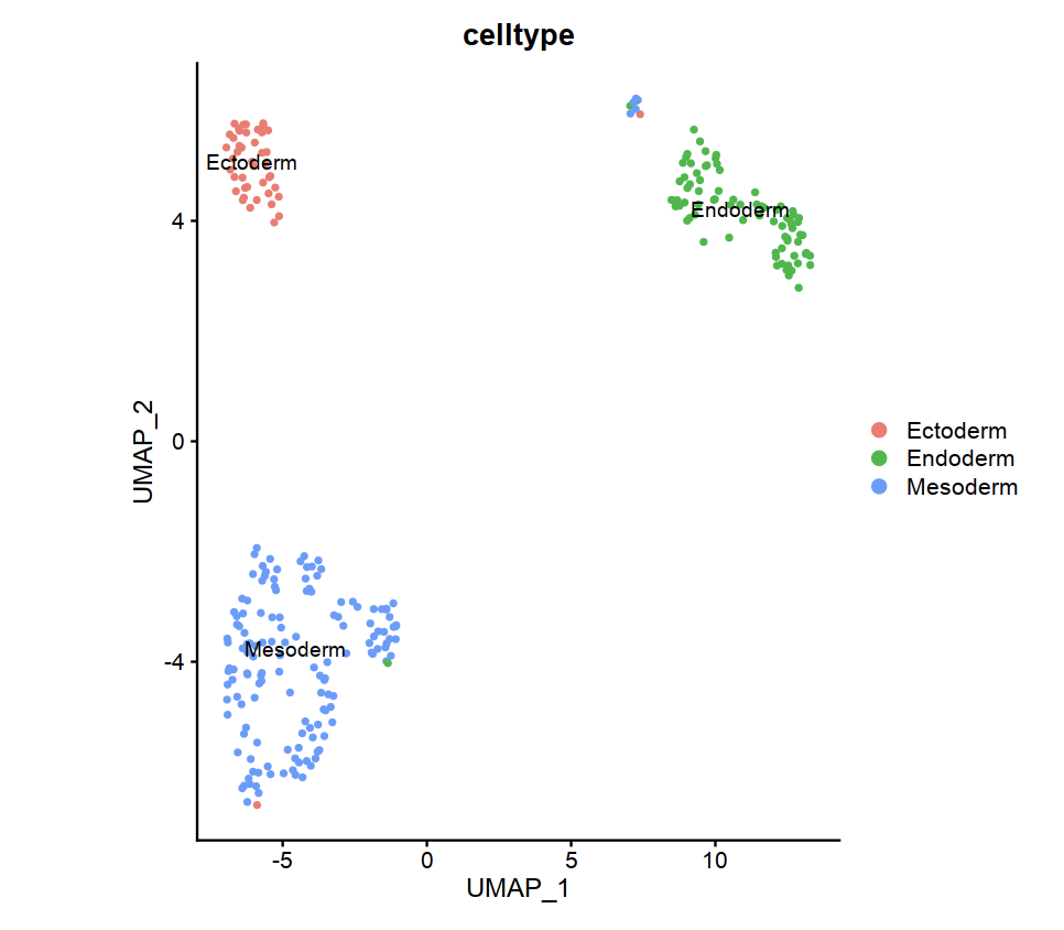
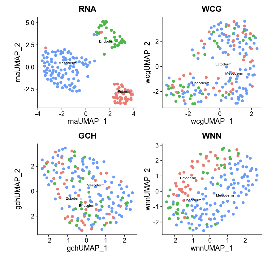
p1 <- DimPlot(seurat, reduction = "umap.rna", group.by = "celltype", label = TRUE, label.size = 2.5, pt.size = 2, repel = TRUE) + ggtitle("RNA")
p2 <- DimPlot(seurat, reduction = "umap.gch", group.by = "celltype", label = TRUE, label.size = 2.5, pt.size = 2, repel = TRUE) + ggtitle("GCH")
p3 <- DimPlot(seurat, reduction = "wnn.umap", group.by = "celltype", label = TRUE, label.size = 2.5, pt.size = 2, repel = TRUE) + ggtitle("WNN")
p1 + p2 +p3  & theme(plot.title = element_text(hjust = 0.5))
dev.off()

# RNA analysis
DefaultAssay(seurat) <- "RNA"
seurat <- SCTransform(seurat, verbose = FALSE) %>% RunPCA() %>% RunUMAP(dims = 1:50, reduction.name = 'umap.rna', reduction.key = 'rnaUMAP_')
# WCG analysis
# We exclude the first dimension as this is typically correlated with sequencing depth
DefaultAssay(seurat) <- "WCG"
seurat <- RunTFIDF(seurat)
seurat <- FindTopFeatures(seurat, min.cutoff = 'q90')
seurat <- RunSVD(seurat)
seurat <- RunUMAP(seurat, reduction = 'lsi', dims = 2:50, reduction.name = "umap.wcg", reduction.key = "wcgUMAP_")

# RNA+WCG
DefaultAssay(seurat) <- "RNA"
seurat <- FindMultiModalNeighbors(seurat, reduction.list = list("pca", "lsi"), dims.list = list(1:50, 2:50),knn.range = 170,sd.scale = 1,k.nn = 30)
seurat <- RunUMAP(seurat, nn.name = "weighted.nn", reduction.name = "wnn.umap", reduction.key = "wnnUMAP_")
seurat <- FindClusters(seurat, graph.name = "wsnn", algorithm = 3, verbose = FALSE)

pdf("WCG+RNA.pdf",width = 10,height = 5)
p1 <- DimPlot(seurat, reduction = "umap.rna", group.by = "celltype", label = TRUE, label.size = 2.5, pt.size = 2, repel = TRUE) + ggtitle("RNA")
p2 <- DimPlot(seurat, reduction = "umap.wcg", group.by = "celltype", label = TRUE, label.size = 2.5, pt.size = 2, repel = TRUE) + ggtitle("WCG")
p3 <- DimPlot(seurat, reduction = "wnn.umap", group.by = "celltype", label = TRUE, label.size = 2.5, pt.size = 2, repel = TRUE) + ggtitle("WNN")
p1 + p2 +p3  & theme(plot.title = element_text(hjust = 0.5))
dev.off()

Spatial multi-omics analysis

library(reticulate)
library(data.table)
library(dplyr)
library(ggplot2)
library(Seurat)
library(Matrix)
library(Giotto)
library(Signac)
np <- import("numpy")
scipy <-import("scipy")

temp_dir = getwd()
temp_dir = '~/Temp/'
myinstructions = createGiottoInstructions(save_dir = temp_dir,
                                          save_plot = TRUE,
                                          show_plot = FALSE)

# initialize spatial expression matrix
expr =  scipy$sparse$load_npz('../STRIDE/WCG_methy_mat.npz')
row = read.csv("../STRIDE/WCG_methy_mat_row.txt",header = FALSE)
spa_loc = read.table("Spa_location_Emb1z5.txt",sep = "\t")
rownames(expr) = row$V1
colnames(expr) = rownames(spa_loc)

signac <- CreateAssayObject(counts = expr)
signac <- RunTFIDF(signac)
signac <- FindTopFeatures(signac, min.cutoff = "q90")
rownames(expr) <- rownames(signac@data)
# giotto object
seqfish_mini <- createGiottoObject(raw_exprs = expr,
                                   norm_expr = signac@data,
                                   spatial_locs = spa_loc,
                                   instructions = myinstructions,cores = 3)

## spatial grid
seqfish_mini <- createSpatialGrid(gobject = seqfish_mini,
                             sdimx_stepsize = 0.5,
                             sdimy_stepsize = 0.5,minimum_padding = 0.1)

spatPlot(gobject = seqfish_mini, show_grid = T, point_size = 1.5,
         save_param = c(save_name = '8_a_grid'))


## delaunay network: stats + creation
plotStatDelaunayNetwork(gobject = seqfish_mini, maximum_distance = 400, save_plot = F)
seqfish_mini = createSpatialNetwork(gobject = seqfish_mini, minimum_k = 10, maximum_distance_delaunay = 400)


km_spatialgenes = binSpect(seqfish_mini, bin_method = 'rank', cores = 3)
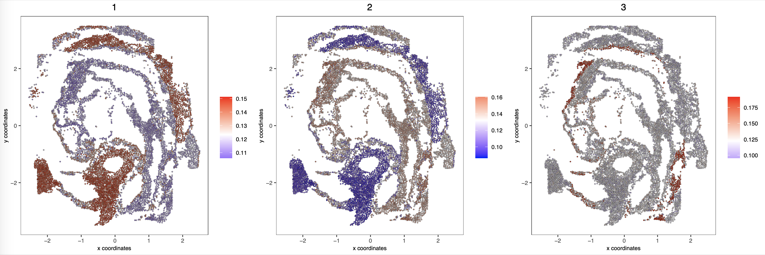
spatGenePlot(seqfish_mini, expression_values = 'normalized', genes = km_spatialgenes[c(1:4),]$genes,
             point_shape = 'border', point_border_stroke = 0.1,
             show_network = F, network_color = 'lightgrey', point_size = 0.8,
             cow_n_col = 2,
             save_param = list(save_name = '10_a_spatialgenes_km'))


# 1. calculate spatial correlation scores
ext_spatial_genes = km_spatialgenes[1:2500]$genes
spat_cor_netw_DT = detectSpatialCorGenes(seqfish_mini,
                                         method = 'network',
                                         spatial_network_name = 'Delaunay_network',
                                         subset_genes = ext_spatial_genes)

# 2. cluster correlation scores
spat_cor_netw_DT = clusterSpatialCorGenes(spat_cor_netw_DT,
                                          name = 'spat_netw_clus', k = 2)
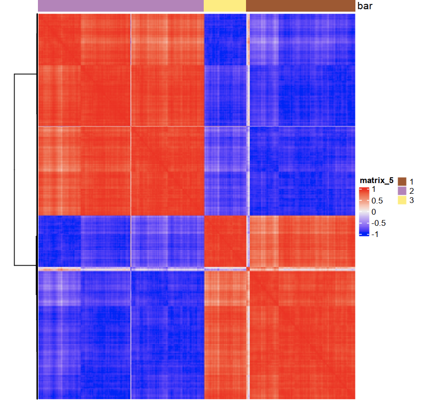
heatmSpatialCorGenes(seqfish_mini, spatCorObject = spat_cor_netw_DT,
                     use_clus_name = 'spat_netw_clus')

netw_ranks = rankSpatialCorGroups(seqfish_mini,
                                  spatCorObject = spat_cor_netw_DT,
                                  use_clus_name = 'spat_netw_clus')

cluster_genes_DT = showSpatialCorGenes(spat_cor_netw_DT,
                                       use_clus_name = 'spat_netw_clus',
                                       show_top_genes = 1)
cluster_genes = cluster_genes_DT$clus; names(cluster_genes) = cluster_genes_DT$gene_ID

seqfish_mini = createMetagenes(seqfish_mini, gene_clusters = cluster_genes, name = 'cluster_metagene')
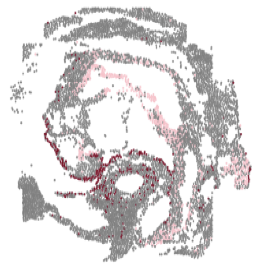
spatCellPlot(seqfish_mini,
             spat_enr_names = 'cluster_metagene',
             cell_annotation_values = netw_ranks$clusters,
             point_size = 0.7, cow_n_col = 3)